| |
Chapter 4. Interplanetary Trajectories
- Objectives:
- Upon completion of this chapter you will be able to
describe the use of Hohmann transfer orbits in general terms and how
spacecraft use them for interplanetary travel. You will be able to describe
the general concept of exchanging angular momentum between planets and
spacecraft to achieve gravity assist trajectories.
When travelling among the
planets, it's a good idea to minimize the propellant mass needed by your
spacecraft and its launch vehicle. That way, such a flight is possible with
current launch capabilities, and costs will not be prohibitive. The amount of
propellant needed depends largely on what route you choose. Trajectories that by
their nature need a minimum of propellant are therefore of great interest.
Hohmann Transfer Orbits
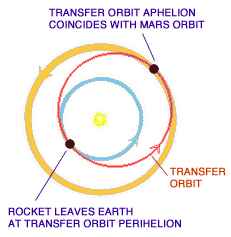
To launch a spacecraft from Earth to an outer planet
such as Mars using the least propellant possible, first consider that the
spacecraft is already in solar orbit as it sits on the launch pad. This existing
solar orbit must be adjusted to cause it to take the spacecraft to Mars: The
desired orbit's perihelion (closest approach to the sun) will be at the distance
of Earth's orbit, and the aphelion (farthest distance from the sun) will be at
the distance of Mars' orbit. This is called a Hohmann Transfer orbit. The
portion of the solar orbit that takes the spacecraft from Earth to Mars is
called its trajectory.
From the above, we know that the task is to increase
the apoapsis (aphelion) of the spacecraft's present solar orbit. Recall from
Chapter 3...
| A spacecraft's apoapsis
altitude can be raised by increasing the spacecraft's energy at periapsis.
|
Well, the spacecraft is already at periapsis. So the
spacecraft lifts off the launch pad, rises above Earth's atmosphere, and uses
its rocket to accelerate in the direction of Earth's revolution around the
sun to the extent that the energy added here at periapsis (perihelion) will
cause its new orbit to have an aphelion equal to Mars' orbit.
After this brief acceleration away from Earth, the
spacecraft has achieved its new orbit, and it simply coasts the rest of the way.
The launch phase is covered further in Chapter 14.
Earth to Mars via Least Energy Orbit
Getting to the planet Mars, rather than just to its
orbit, requires that the spacecraft be inserted into its interplanetary
trajectory at the correct time so it will arrive at the Martian orbit when Mars
will be there. This task might be compared to throwing a dart at a moving
target. You have to lead the aim point by just the right amount to hit the
target. The opportunity to launch a spacecraft on a transfer orbit to Mars
occurs about every 25 months.
To be captured into a Martian orbit, the spacecraft
must then decelerate relative to Mars using a retrograde rocket burn or some
other means. To land on Mars, the spacecraft must decelerate even further using
a retrograde burn to the extent that the lowest point of its Martian orbit will
intercept the surface of Mars. Since Mars has an atmosphere, final deceleration
may also be performed by aerodynamic braking direct from the interplanetary
trajectory, and/or a parachute, and/or further retrograde burns.
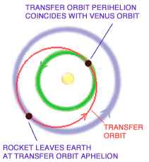
To launch a spacecraft from Earth to an
inner planet such as Venus using least propellant, its existing solar orbit (as
it sits on the launch pad) must be adjusted so that it will take it to Venus. In
other words, the spacecraft's aphelion is already the distance of Earth's orbit,
and the perihelion will be on the orbit of Venus.
This time, the task is to decrease
the periapsis (perihelion) of the spacecraft's present solar orbit. Recall
from Chapter 3...
| A spacecraft's periapsis
altitude can be lowered by decreasing the spacecraft's energy at apoapsis.
|
To achieve this, the spacecraft lifts
off of the launch pad, rises above Earth's atmosphere, and uses its rocket to
accelerate opposite the direction of Earth's revolution around the sun,
thereby decreasing its orbital energy while here at apoapsis (aphelion)
to the extent that its new orbit will have a perihelion equal to the distance of
Venus's orbit.
Of course the spacecraft will continue
going in the same direction as Earth orbits the sun, but a little slower now. To
get to Venus, rather than just to its orbit, again requires that the spacecraft
be inserted into its interplanetary trajectory at the correct time so it will
arrive at the Venusian orbit when Venus is there. Venus launch opportunities
occur about every 19 months.
Type I and II Trajectories
If the interplanetary trajectory carries the spacecraft
less than 180 degrees around the sun, it's called a Type-I Trajectory. If the
trajectory carries it 180 degrees or more around the sun, it's called a Type-II.
Gravity Assist Trajectories
Chapter 1 pointed out that the planets retain most of
the solar system's angular momentum. This momentum can be tapped to accelerate
spacecraft on so-called "gravity-assist" trajectories. It is commonly stated in
the news media that spacecraft such as Voyager, Galileo, and Cassini use a
planet's gravity during a flyby to slingshot it farther into space. How does
this work? By using gravity to tap into the planet's tremendous angular
momentum.
In a gravity-assist trajectory, angular momentum is
transferred from the orbiting planet to a spacecraft approaching from behind the
planet in its progress about the sun.
Note: experimenters and
educators may be interested in the
Gravity Assist
Mechanical Simulator, a device you can build and operate to gain an
intuitive understanding of how gravity assist trajectories work. The linked
pages include an illustrated "primer"
on gravity assist.
 Consider Voyager 2, which toured the Jovian planets. The spacecraft was launched
on a Type-II Hohmann transfer orbit to Jupiter. Had Jupiter not been there at
the time of the spacecraft's arrival, the spacecraft would have fallen back
toward the sun, and would have remained in elliptical orbit as long as no other
forces acted upon it. Perihelion would have been at 1 AU, and aphelion at
Jupiter's distance of about 5 AU.
Consider Voyager 2, which toured the Jovian planets. The spacecraft was launched
on a Type-II Hohmann transfer orbit to Jupiter. Had Jupiter not been there at
the time of the spacecraft's arrival, the spacecraft would have fallen back
toward the sun, and would have remained in elliptical orbit as long as no other
forces acted upon it. Perihelion would have been at 1 AU, and aphelion at
Jupiter's distance of about 5 AU.
However, Voyager's arrival at
Jupiter was carefully timed so that it would pass behind Jupiter in its orbit
around the sun. As the spacecraft came into Jupiter's gravitational influence,
it fell toward Jupiter, increasing its speed toward maximum at closest approach
to Jupiter. Since all masses in the universe attract each other, Jupiter sped up
the spacecraft substantially, and the spacecraft tugged on Jupiter,
causing the massive planet to actually lose some of its orbital energy.
The spacecraft passed on by
Jupiter since Voyager's velocity was greater than Jupiter's escape velocity, and
of course it slowed down again relative to Jupiter as it climbed out of the huge
gravitational field. The speed component of its Jupiter-relative velocity
outbound dropped to the same as that on its inbound leg.
But relative to the sun, it never
slowed all the way to its initial Jupiter approach speed. It left the Jovian
environs carrying an increase in angular momentum stolen from Jupiter. Jupiter's
gravity served to connect the spacecraft with the planet's ample reserve of
angular momentum. This technique was repeated at Saturn and Uranus.
Voyager 2 Gravity Assist
Velocity Changes
| Voyager 2 leaves Earth at about 36 km/s
relative to the sun. Climbing out, it loses much of the initial velocity the
launch vehicle provided. Nearing Jupiter, its speed is increased by the
planet's gravity, and the spacecraft's velocity exceeds solar system escape
velocity. Voyager departs Jupiter with more sun-relative velocity than it
had on arrival. The same is seen at Saturn and Uranus. The Neptune flyby
design put Voyager close by Neptune's moon Triton rather than attain more
speed. Diagram courtesy Steve Matousek, JPL. |
|
The same can be said of a
baseball's acceleration when hit by a bat: angular momentum is transferred from
the bat to the slower-moving ball. The bat is slowed down in its "orbit" about
the batter, accelerating the ball greatly. The bat connects to the ball not with
the force of gravity from behind as was the case with a spacecraft, but with
direct mechanical force (electrical force, on the molecular scale, if you
prefer) at the front of the bat in its travel about the batter, translating
angular momentum from the bat into a high velocity for the ball.
(Of course in the analogy a
planet has an attractive force and the bat has a repulsive force, thus Voyager
must approach Jupiter from a direction opposite Jupiter's trajectory and the
ball approaches the bat from the direction of the bats trajectory.)
 The
vector diagram on the left shows the spacecraft's speed relative to Jupiter
during a gravity-assist flyby. The spacecraft slows to the same velocity going
away that it had coming in, relative to Jupiter, although its direction has
changed. Note also the temporary increase in speed nearing closest approach. The
vector diagram on the left shows the spacecraft's speed relative to Jupiter
during a gravity-assist flyby. The spacecraft slows to the same velocity going
away that it had coming in, relative to Jupiter, although its direction has
changed. Note also the temporary increase in speed nearing closest approach.
When the same situation is viewed
as sun-relative in the diagram below and to the right, we see that Jupiter's
sun-relative orbital velocity is added to the spacecraft's velocity, and the
spacecraft does not lose this component on its way out. Instead, the planet
itself loses the energy. The massive planet's loss is too small to be measured,
but the tiny spacecraft's gain can be very great. Imagine a gnat flying into the
path of a speeding freight train.
Gravity assists can be also used
to decelerate a spacecraft, by flying in front of a body in its orbit, donating
some of the spacecraft's angular momentum to the body. When the Galileo
spacecraft arrived at Jupiter, passing close in front of Jupiter's moon Io in
its orbit, Galileo lost energy in relation to Jupiter, helping it achieve
Jupiter orbit insertion, reducing the propellant needed for orbit insertion by
90 kg.
The gravity assist technique was
championed by Michael Minovitch in the early 1960s, while he was a UCLA graduate
student working during the summers at JPL. Prior to the adoption of the gravity
assist technique, it was believed that travel to the outer solar system would
only be possible by developing extremely powerful launch vehicles using nuclear
reactors to create tremendous thrust, and basically flying larger and larger
Hohmann transfers.
An interesting fact to consider
is that even though a spacecraft may double its speed as the result of a gravity
assist, it feels no acceleration at all. If you were aboard Voyager 2 when it
more than doubled its speed with gravity assists in the outer solar system, you
would feel only a continuous sense of falling. No acceleration. This is due to
the balanced tradeoff of angular momentum brokered by the planet's -- and the
spacecraft's -- gravitation.
Enter the Ion Engine
 All
of the above discussion of interplanetary trajectories is based on the use of
today's system of chemical rockets, in which a launch vehicle provides nearly
all of the spacecraft's propulsive energy. A few times a year the spacecraft may
fire short bursts from its chemical rocket thrusters for small adjustments in
trajectory. Otherwise, the spacecraft is in free-fall, coasting all the way to
its destination. Gravity assists may also provide short periods wherein the
spacecraft's trajectory undergoes a change. All
of the above discussion of interplanetary trajectories is based on the use of
today's system of chemical rockets, in which a launch vehicle provides nearly
all of the spacecraft's propulsive energy. A few times a year the spacecraft may
fire short bursts from its chemical rocket thrusters for small adjustments in
trajectory. Otherwise, the spacecraft is in free-fall, coasting all the way to
its destination. Gravity assists may also provide short periods wherein the
spacecraft's trajectory undergoes a change.
But ion electric propulsion, as
demonstrated in interplanetary flight by Deep Space 1, works differently.
Instead of short bursts of relatively powerful thrust, electric propulsion uses
a more gentle thrust continuously over periods of months or even years. It
offers a gain in efficiency of an order of magnitude over chemical propulsion
for those missions of long enough duration to use the technology. Ion engines
are discussed further under
Propulsion in Chapter 11.
Click the image above for more
information about Deep Space 1. The Japan Aerospace Exploration Agency's
asteroid explorer
HAYABUSA also employs an ion engine.
Even ion-electric propelled
spacecraft need to launch using chemical rockets, but because of their
efficiency they can be less massive, and require less powerful (and less
expensive) launch vehicles. Initially, then, the trajectory of an ion-propelled
craft may look like the Hohmann transfer orbit. But over long periods of
continuously operating an electric engine, the trajectory will no longer be a
purely ballistic arc.
For Further Study
Select the "Links" section below
for additional references, including mathe
Chapter 6. Electromagnetic Phenomena CONTINUED
Radio Frequencies
Abbreviations such as kHz and GHz are all listed in the Glossary and are
also treated under Units of Measure (see the menu bar below).
Electromagnetic radiation with frequencies between about 10 kHz and 100
GHz are referred to as radio frequencies (RF). Radio frequencies are divided
into groups that have similar characteristics, called "bands," such as
"S-band," "X-band," etc. The bands are further divided into small ranges of
frequencies called "channels," some of which are allocated for the use of
deep space telecommunications. Many deep-space vehicles use channels in the
S-band and X-band range which are in the neighborhood of 2 to 10 GHz. These
frequencies are among those referred to as microwaves, because their
wavelength is short, on the order of centimeters. The microwave oven takes
its name from this range of radio frequencies. Deep space telecommunications
systems are being developed for use on the even higher frequency K-band.
This table lists some RF band definitions for illustration. Band
definitions may vary among different sources and according to various users.
These are "ballpark" values, intended to offer perspective, since band
definitions have not evolved to follow any simple alphabetical sequence. For
example, notice that while "L-Band" represents lower frequencies than
"S-Band," "Q-Band" represents higher frequencies than "S-Band."
| Band |
Approx. Range of
Wavelengths (cm) |
Approximate
Frequencies |
| UHF |
100 - 10 |
300 - 3000 MHz |
| L |
30 - 15 |
1 - 2 GHz |
| S |
15 - 7.5 |
2 - 4 GHz |
| C |
7.5 - 3.75 |
4 - 8 GHz |
| X |
3.75 - 2.4 |
8 - 12 GHz |
| K |
2.4 - 0.75 |
12 - 40 GHz |
| Q |
0.75 - 0.6 |
40 - 50 GHz |
| V |
0.6 - 0.4 |
50 - 80 GHz |
| W |
0.4 - 0.3 |
80 - 90 GHz |
| Within K-band, spacecraft may operate communications,
radio science, or radar equipment at Ku-band in the neighborhood of 15
to 17 GHz and Ka-band around 20 to 30 GHz. |
The Whole Spectrum
Bring up
this
page to study a table of the entire electromagnetic spectrum. The table
shows frequency and wavelength, common names such as "light" and "gamma
rays," size examples, and any attenuation effects in Earth's environment as
discussed below.
Atmospheric Transparency
Because of the absorption phenomenon, observations are impossible at
certain wavelengths from the surface of Earth, since they are absorbed by
the Earth's atmosphere. There are a few "windows" in its absorption
characteristics that make it possible to see visible light and receive many
radio frequencies, for example, but the atmosphere presents an opaque
barrier to much of the electromagnetic spectrum.
Even though the atmosphere is transparent at X-band frequencies, there is
a problem when liquid or solid water is present. Water exhibits noise at
X-band frequencies, so precipitation at a receiving site increases the
system noise temperature, and this can drive the SNR too low to permit
communications reception.
In addition to the natural interference that comes from
water at X-band, there may be other sources of noise, such as human-made
radio interference. Welding operations on an antenna produce a wide spectrum
of radio noise at close proximity to the receiver. Many Earth-orbiting
spacecraft have strong downlinks near the frequency of signals from deep
space. Goldstone Solar System Radar (described further in this chapter) uses
a very powerful transmitter, which can interfere with reception at a nearby
station. Whatever the source of radio frequency interference (RFI), its
effect is to increase the noise, thereby decreasing the SNR and making it
more difficult, or impossible, to receive valid data from a deep-space
craft.
Spectroscopy
The study of the production, measurement, and interpretation of
electromagnetic spectra is known as spectroscopy. This branch of science
pertains to space exploration in many different ways. It can provide such
diverse information as the chemical composition of an object, the speed of
an object's travel, its temperature, and more -- information that cannot be
gleaned from photographs or other means.
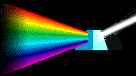 For
purposes of introduction, imagine sunlight passing through a glass prism,
creating a rainbow, called the spectrum. Each band of color visible in this
spectrum is actually composed of a very large number of individual
wavelengths of light which cannot be individually discerned by the human
eye, but which are detectable by sensitive instruments such as spectrometers
and spectrographs. For
purposes of introduction, imagine sunlight passing through a glass prism,
creating a rainbow, called the spectrum. Each band of color visible in this
spectrum is actually composed of a very large number of individual
wavelengths of light which cannot be individually discerned by the human
eye, but which are detectable by sensitive instruments such as spectrometers
and spectrographs.
 Suppose
instead of green all you find is a dark "line" where green should be. You
might assume something had absorbed all the "green" wavelengths out of the
incoming light. This can happen. By studying the brightness of individual
wavelengths from a natural source, and comparing them to the results of
laboratory experiments, many substances can be identified that lie in the
path from the light source to the observer, each absorbing particular
wavelengths, in a characteristic manner. Suppose
instead of green all you find is a dark "line" where green should be. You
might assume something had absorbed all the "green" wavelengths out of the
incoming light. This can happen. By studying the brightness of individual
wavelengths from a natural source, and comparing them to the results of
laboratory experiments, many substances can be identified that lie in the
path from the light source to the observer, each absorbing particular
wavelengths, in a characteristic manner.
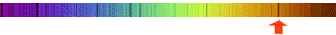
Dark absorption lines in the sun's spectrum and that of other stars are
called Fraunhofer lines after
Joseph von Fraunhofer (1787-1826) who observed them in 1817. The image
below shows a segment of the solar spectrum, in which many such lines can be
seen. The prominent line above the arrow results from hydrogen in the sun's
atmosphere absorbing energy at a wavelength of 6563 Angstroms. This is
called the hydrogen alpha line.
On the other hand, bright lines in a spectrum (not illustrated here)
represent a particularly strong emission of radiation produced by the source
at a particular wavelength.
Spectroscopy is not limited to the band of visible light, but is commonly
applied to infrared, ultraviolet, and many other parts of the
whole
spectrum of electromagnetic energy.
| In 1859,
Gustav Kirchhoff (1824-1887) described three laws of spectral
analysis:
- A luminous (glowing) solid or liquid emits
light of all wavelengths (white light), thus producing a continuous
spectrum.
- A rarefied luminous gas emits light whose
spectrum shows bright lines (indicating light at specific
wavelengths), and sometimes a faint superimposed continuous spectrum.
- If the white light from a luminous source is
passed through a gas, the gas may absorb certain wavelengths from the
continuous spectrum so that those wavelengths will be missing or
diminished in its spectrum, thus producing dark lines.
|
By studying emission and absorption features in the spectra of stars, in
the spectra of sunlight reflected off the surfaces of planets, rings, and
satellites, and in the spectra of starlight passing through planetary
atmospheres, much can be learned about these bodies. This is why spectral
instruments are flown on spacecraft.
Historically, spectral observations have taken the form of photographic
prints showing spectral bands with light and dark lines. Modern instruments
(discussed
 again under Chapter 12) produce their high-resolution results in the form of
X-Y graphic plots, whose peaks and valleys reveal intensity (brightness) on
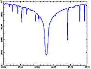
the vertical axis versus wavelength along the horizontal. Peaks of high
intensity on such a plot represent bright spectral lines (not seen in this
illustration), and troughs of low intensity represent the dark lines.
again under Chapter 12) produce their high-resolution results in the form of
X-Y graphic plots, whose peaks and valleys reveal intensity (brightness) on
the vertical axis versus wavelength along the horizontal. Peaks of high
intensity on such a plot represent bright spectral lines (not seen in this
illustration), and troughs of low intensity represent the dark lines.
This plot, reproduced courtesy of the
Institut
National des Sciences de l'Univers / Observatoire de Paris, shows
details surrounding the dip in brightness centered at the hydrogen-alpha
line of 6563 Å which is indicated by the dark line above the red arrow in
the spectral image above. The whole plot spans 25 Å of wavelength
horizontally. Click the image for a larger view.
Spectral observations of distant supernovae (exploding stars) provide
data for astrophysicists to understand the supernova process, and to
categorize the various supernova types. Supernovae can be occasionally found
in extremely distant galaxies. Recognizing their
spectral signature is an important step in measuring the size of the
universe, based on knowing the original brightness of a supernova and
comparing that with the observed brightness across the distance. |
matical tutorials and example problems.
Chapter 6. Electromagnetic Phenomena
CONTINUED
The Doppler Effect

CLICK IMAGE TO
START / STOP ANIMATION
|
Regardless of the frequency of a source of electromagnetic waves, they
are subject to the Doppler effect. The effect was discovered by the Austrian
mathematician and physicist
Christian Doppler (1803-1853). It causes the observed frequency of any
source (sound, radio, light, etc.) to differ from the radiated frequency of
the source if there is motion that is increasing or decreasing the distance
between the source and the observer. The effect is readily observable as
variation in the pitch of
sound between a moving source and a stationary observer, or vice-versa.
Consider the following:
1. When the distance
between the source and receiver of electromagnetic waves remains constant,
the frequency of the source and received wave forms is the same.
This is illustrated at right. The waveform at the
top represents the source, and the one at the bottom represents the received
signal. Since the source and the receiver are not moving toward or away from
each other, the received signal appears the same as the source.
2. When the
distance between the source and receiver of electromagnetic waves is
increasing, the frequency of the received wave forms appears to be
lower than the actual frequency of the source wave form. Each time the
source has completed a wave, it has also moved farther away from the
receiver, so the waves arrive less frequently.
3. When the
distance is decreasing, the frequency of the received wave form will be
higher than the source wave form. Since the source is getting closer,
the waves arrive more frequently.
Cases 2 and 3 are illustrated below. Notice that
when the receiver is in motion toward or away from the source, the waveform
at the receiver (the lower waveform) changes. It only changes, though, while
there is actual motion toward or away; when it stops, the received waveform
appears the same as the source.
|
|
CLICK
IMAGE TO START / STOP ANIMATION
|
The Doppler effect is routinely measured in the
frequency of the signals received by ground receiving stations when tracking
spacecraft. The increasing or decreasing distances between the spacecraft
and the ground station may be caused by a combination of the spacecraft's
trajectory, its orbit around a planet, Earth's revolution about the sun, and
Earth's daily rotation on its axis. A spacecraft approaching Earth will add
a positive frequency bias to the received signal. However, if it flies by
Earth, the received Doppler bias will become zero as it passes Earth, and
then become negative as the spacecraft moves away from Earth.
A spacecraft's revolutions around another planet
such as Mars adds alternating positive and negative frequency biases to the
received signal, as the spacecraft first moves toward and then away from
Earth.
The Earth's daily rotation adds a positive
frequency bias to the received signal as the spacecraft rises in the
east at a particular tracking station, and it adds a negative
frequency bias to the received signal as the spacecraft sets in the
west.
The Earth's revolution about the sun adds a
positive frequency bias to the received signal during that portion of the
year when the Earth is moving toward the spacecraft, and it adds a negative
frequency bias during the part of the year when the Earth is moving away.
Differenced Doppler
If two widely-separated tracking stations on Earth
observe a single spacecraft in orbit about another planet, they will each
have a slightly different view of the moving spacecraft, and there will be a
slight difference in the amount of Doppler shift observed by each station.
For example, if one station has a view exactly edge-on to the spacecraft's
orbital plane, the other station would have a view slightly to one side of
that plane. Information can be extracted from the differencing of the two
received signals.
Data obtained from two stations in this way can be
combined and interpreted to fully describe the spacecraft's arc through
space in three dimensions, rather than just providing a single toward or
away component. This data type, differenced Doppler, is a useful form of
navigation data that can yield a very high degree of spatial resolution. It
is further discussed in Chapter 13, Spacecraft Navigation.
Refraction
Refraction is the deflection or bending of electromagnetic waves when
they pass from one kind of transparent medium into another. The index of
refraction of a material is the ratio of the speed of light in a vacuum
to the speed of light in the material. Electromagnetic waves passing from
one medium into another of a differing index of refraction will be bent in
their direction of travel. In 1621, Dutch physicist Willebrord Snell
(1591-1626), determined the
angular relationships of light passing from one transparent medium to
another.
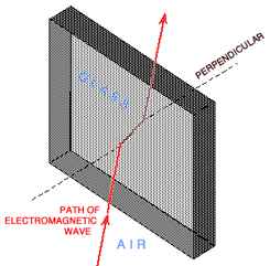
Air and glass have different indices of refraction. Therefore, the path
of electromagnetic waves moving from air to glass at an angle will be bent
toward the perpendicular as they travel into the glass. Likewise, the path
will be bent to the same extent away from the perpendicular when they exit
the other side of glass.
Refraction is responsible for many useful devices which bend light in
carefully determined ways, from
eyeglasses to refracting
telescope
lenses.
Refraction can cause
 illusions.
This pencil appears to be discontinuous at the boundary of air and water.
Spacecraft may appear to be in different locations in the sky than they
really are. illusions.
This pencil appears to be discontinuous at the boundary of air and water.
Spacecraft may appear to be in different locations in the sky than they
really are.
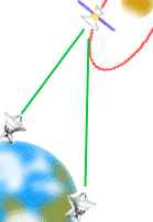
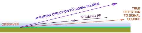
Electromagnetic waves entering Earth's atmosphere from space are bent by
refraction. Atmospheric refraction is greatest for signals near the horizon
where they come in at the lowest angle. The apparent altitude of the signal
source can be on the order of half a degree higher than its true height. As
Earth rotates and the object gains altitude, the refraction effect reduces,
becoming zero at the zenith (directly overhead). Refraction's effect on the
Sun adds about 5 minutes of time to the daylight at equatorial latitudes,
since it appears higher in the sky than it actually is.
Refraction in Earth's Atmosphere
Angles exaggerated for clarity.
If the signal from a spacecraft goes through the atmosphere of another
planet, the signals leaving the spacecraft will be bent by the atmosphere of
that planet. This bending will cause the apparent occultation, that is,
going behind the planet, to occur later than otherwise expected, and to exit
from occultation prior to when otherwise expected. Ground processing of the
received signals reveals the extent of atmospheric bending, and also of
absorption at specific frequencies and other modifications. These provide a
basis for inferring the composition and structure of a planet's atmosphere.
|
|
